the Creative Commons Attribution 3.0 License.
the Creative Commons Attribution 3.0 License.
Real-time hydraulic interval state estimation for water transport networks: a case study
Stelios G. Vrachimis
Demetrios G. Eliades
Marios M. Polycarpou
Hydraulic state estimation in water distribution networks is the task of estimating water flows and pressures in the pipes and nodes of the network based on some sensor measurements. This requires a model of the network as well as knowledge of demand outflow and tank water levels. Due to modeling and measurement uncertainty, standard state estimation may result in inaccurate hydraulic estimates without any measure of the estimation error. This paper describes a methodology for generating hydraulic state bounding estimates based on interval bounds on the parametric and measurement uncertainties. The estimation error bounds provided by this method can be applied to determine the existence of unaccounted-for water in water distribution networks. As a case study, the method is applied to a modified transport network in Cyprus, using actual data in real time.


Hydraulic state estimation in water distribution networks (WDNs) is a challenging task due to the presence of modeling uncertainties, such as structural uncertainty introduced by skeletonization of the network, parameter uncertainty of pipe roughness coefficients and uncertainty in water demands. While this last uncertainty can be reduced by the use of real-time flow measurements, these measurements come with their own instrument uncertainties and noise (Hutton et al., 2014).
In standard state estimation techniques, statistical characterization of sensor measurement error is needed to give more weight to measurements originating from more accurate sensors. Using the weighted least squares method, the nodal demands are adjusted to fit the constraints imposed by the measurements and produce the most probable state estimate (Davidson and Bouchart, 2006). Another approach is the Kalman filter (KF) method which provides a solution for the network state based on the available measurements. The standard KF performs poorly in nonlinear looped WDN due to the use of a linearized system model (Kang et al., 2009). Overall, the above methods generate a point in state space and are referred to as point state estimation (Andersen et al., 2001).
Most point state estimation methods assume a known statistical characterization of the measurement error. This could lead to significant estimation errors, especially in the case when pseudo-measurements are used, which are estimates determined from population densities and historical data. The use of pseudo-measurements may be necessary when there are not enough sensors to guarantee the observability of the network. In this case, no measure of the estimation error is available. Additionally, in order for point state estimation methods to produce feasible solutions, model calibration is required a priori or during state estimation (Kang and Lansey, 2011; Savic et al., 2009).
An alternative approach for the representation of measurement and model parameter uncertainty is the use of bounds. In contrast to traditional point state estimation methods, the use of bounding uncertainty can provide upper and lower bounds on the state variables. This method is referred to as interval state estimation. In this work a hydraulic interval state estimation methodology is described and its use is demonstrated with a case study of a modified transport network of a water utility in Cyprus. An application of this method for determining the existence of unaccounted-for water in the network is presented.
The use of measurement bounds for the representation of measurement uncertainty and their incorporation into the state estimation cost function was introduced by Bargiela and Hainsworth (1989). Interval state estimation was developed by Gabrys and Bargiela (1997) as the so-called set-bounded state estimation problem. An implicit state estimation technique for leakage detection for an idealized grid network under steady conditions was presented by Andersen and Powell (2000). A straightforward method for interval state estimation is the use of Monte Carlo simulations (MCS), which under some assumptions converge to the true uncertainty bounds by randomly generating and evaluating a large number of parameter sets or realizations (Eliades et al., 2015). The interval-based approach used in this paper has the advantage of calculating algorithmically the bounded state estimates in a way that guarantees the inclusion of the true state. MCS, even with a large number of simulations, cannot guarantee that all possible cases will be simulated. The applicability of the proposed algorithm is thus suitable for event and fault-detection methodologies that require strict bounds on state estimates.
In many applications, such as leakage detection and contamination detection, the derivation of a range of possible values for the state of the WDN provides useful information for event and fault-detection methodologies. Hydraulic state bounds can be used to generate bounds on chlorine concentration in the water network or other chemicals in the water, by taking into consideration the uncertainty in decay rate (Vrachimis et al., 2015). When additionally this bounded estimate is generated in real time, it helps to reduce the time of detecting water leakages and prevent catastrophic scenarios such as water contamination.
The paper is organized as follows: Sect. 2 formulates the problem of hydraulic state estimation and describes a methodology to solve this problem based on the Iterative Hydraulic Interval State Estimation (IHISE) algorithm. In Sect. 3, a case study is presented in which this method is applied to a modified real transport network. Finally, we discuss the application of this method for determining the existence of unaccounted-for water in the network.
A water transport network is modeled using a directed graph, for which nodes represent water sources, junctions of pipes and water demand locations, and the links represent pipes. Each pipe is indicated by the index j, where and np is the number of pipes. These are characterized by pipe length, diameter and roughness coefficient, parameters which are generally assumed known. Pipe parameters are used to compute the Hazen–Williams (H–W) resistance coefficients rj, which are in turn used to formulate the energy conservation equations of a water network (Boulos et al., 2006).
Modeling uncertainty in a WDN is considered in this work to arise from insufficient knowledge of pipe parameters. The uncertain parameters are represented using intervals, with the actual value of the parameter being within a corresponding interval. For notational convenience, the parameters representing intervals will be denoted with a tilde. Any uncertain parameters in pipe j will be included in . The interval parameter is the uncertain H–W coefficient for pipe j, with and being the lower and upper bounds of each coefficient, respectively.
Nodes are indicated by the index i, where and nu is the number of nodes with an unknown head, thus excluding the nodes that represent water sources. In this work we consider water transport networks in which sensors measure all the water demands at nodes, which, typically, are the inflows of district metered areas (DMAs). Measurements arrive at a fixed time interval from sensors that may not be accurate, and each measurement is associated with a certain measurement error. The uncertainty of each measurement is given as a percent error of the measurement, and it is modeled as an interval with the measurement being the mean value of the interval. Measured water demand at node i is then given by the interval , where is the lower bound on water demand and is the upper bound.
The unknown state vector of the WDN is denoted by , where are the unknown heads at nodes, are the water flows in pipes and . These are computed by formulating the conservation of energy and mass equations, as formulated by Todini and Pilati (1987). The matrix formulation for a general looped water distribution system, which also includes the uncertain parameters and variables as intervals (denoted with a tilde), is given by
where is a diagonal matrix containing the nonlinear terms , is the incidence flow matrix that indicates the connectivity of nodes with links, ν=1.852 is a constant associated with the H–W coefficient and is a vector that contains the known heads in each equation. For simplicity, we assume that measurements of the tank levels are available; thus, hext is known.
Equation (1) represents a system of nonlinear equations, which include interval parameters, and it is referred to in the literature as a nonlinear interval parametric (NIP) problem (Kolev, 2014). The objective is to find the smallest interval state vector that contains all the solutions of this system of equations for every value contained in the interval parameters. To solve the NIP problem given in Eq. (1), an algorithmic technique named iterative hydraulic interval state estimation (IHISE) was developed by the authors. The IHISE method comprises five steps: (1) find initial bounds on the state vector x. (2) Use interval linearization to remove nonlinear terms from Eq. (1) and transform them into a system of linear interval parametric (LIP) equations. (3) Formulate a linear program (LP) using the system of LIP equations. (4) Solve the LIP problem. (5) Iteratively tighten the bounds on x and approximate the solution of the NIP problem.
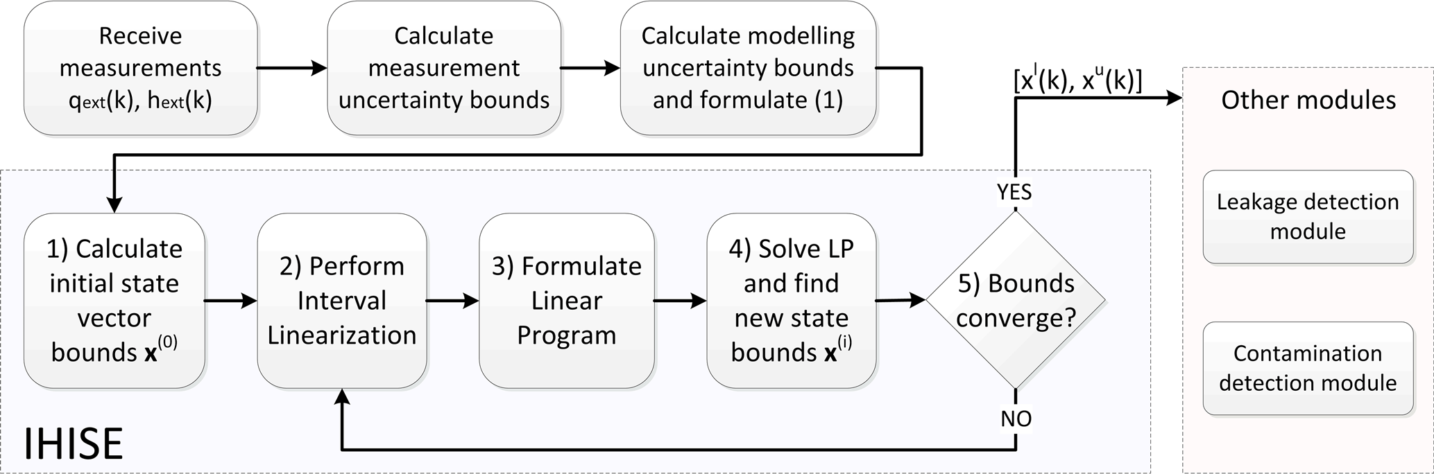
Figure 1 illustrates how this technique is implemented in a real-time framework. At discrete time instant k, the measurements from the sensors in the network are received, which include the water outflow qext(k) and the water level in tanks. The measured tank level at each time instant is used to calculate the known head vector hext(k) of the network. Since these equations only depend on the current time instant k, the discrete time notation is omitted. The uncertainty of these measurements is inserted by converting them into intervals with the measurement as the mean value. The hydraulic equations of Eq. (1) are then formulated using the new measurements. Modeling uncertainty is represented by including the interval parameters in the equations.
The first step of the IHISE algorithm is to impose initial bounds on the state vector x. The initial bounds should be an outer interval solution of Eq. (1) (Kolev, 2014). An outer interval solution includes all the point solutions of Eq. (1), but it is not the smallest possible interval. Bounds on the unknown head vector h can be chosen using physical properties of the network such as the minimum head of each node and the maximum head that pumps and water sources can add to the network. After finding an initial interval for the unknown heads , the special structure of Eq. (1), in which each equation contains only one flow state qi, allows us to use and interval arithmetic to find the initial bounds on the flows .
In the second step, the nonlinear terms present in Eq. (1) need to be linearized in order for the system of equations to be transformed into a LIP problem and solved (Kolev, 2004a). This is achieved using interval linearization (Kolev, 2004b). Given a range of values for the state in which interval linearization will be performed, each of the nonlinear functions is enclosed between two lines and an interval term represents the linearization uncertainty. In the third step, the LIP equations are formulated into a LP with constraints. The interval terms in these equations are transformed into constraints of the LP and a suitable cost function ensures that the solution of this problem will give either the minimum or maximum of a certain state.
To get an interval solution of the whole state vector x, in step four, the LP formulated is solved for all the states by changing the cost function. At the end of this step, an interval solution for the linearized system of equations is derived. The new bounds on state vector x are then checked for convergence in step five. The criterion for convergence is that the relative change in bounds e(m) at iteration m must be smaller than a specified small number ϵ, where ϵ defines the largest allowable absolute error for the calculated bounds of each state, e.g., for flow states ϵ=0.01 (m3 h−1). The relative change in bounds e(m) is computed as follows:
where xu and xl indicate the upper and lower bounds of the state x, respectively. The algorithm then gives the final state bounds calculated as the result. Otherwise, the new bounds are used as initial bounds and the algorithm re-iterates from step two.
This study uses data from a real water transport sub-network in Cyprus. A modified version of the transport network is used, of which an illustrative diagram is shown in Fig. 2. The modified network contains three loops and comprises 9 demand nodes, one water tank and 12 links which represent pipes. Flow sensors (F) are installed at demand nodes, which represent aggregated real measurements at entrances to DMAs, and a water level sensor (L) is installed in the tank. Sensor measurements arrive at fixed 5 min intervals. The tank's water input originates from four water sources, of which three are water dams and one is a desalination unit. The water inflow q0 coming from these sources is measured with a flow sensor. The water outflow q1 of the tank is not directly measured.

3.1 Real-time hydraulic interval state estimation
The implementation of this case study in real time is based on a platform for real-time monitoring of WDN against hydraulic and quality events. A model of the transport network was created as an EPANET input file. Using the platform, one can select the dates with available sensor data and request a state estimation. The available measurements from demand nodes and the level of the tank are then retrieved and a data validation process takes place which replaces missing data.
Sensor measurements have an uncertainty which is defined by the installed sensor's specifications. The measurements given by the flow sensors are within ±2 % of the actual flow at those locations. Modeling uncertainty is also present in the form of pipe parameter uncertainty. For this case study we assumed a total uncertainty of ±2 % in the Hazen–Williams coefficient. The value of this uncertainty may vary, as it is calculated using expert-elicited bounds on the modeled pipe parameters. It is assumed that the network graph is known, and thus structural uncertainty is neglected. This is a valid assumption in transport networks where the structure is known, as it is the network in this case study.
Using the IHISE algorithm, bounds on water flows and pressures in the network are generated using the flow measurements at demand nodes and the tank level measurements, by taking into account measurement and modeling uncertainty. The algorithm needs approximately 4 s to calculate bounds for each hydraulic step, on a personal computer with Intel Core i5-2400 CPU at 3.10 GHz. The bounds converge after eight iterations. The size of bounds does not increase over time because it depends only on the measurements of that specific time step. The effect of accumulating uncertainty due to the dynamic calculation of tank levels does not affect the size of the bounds in this case study, because the tank level is measurable. For illustration purposes, flow and pressure estimates using a real-time EPANET-based state estimator are also generated. The state estimates for a selected pipe and node, accompanied by its corresponding uncertainty bounds generated by the IHISE algorithm, are shown in Fig. 3.
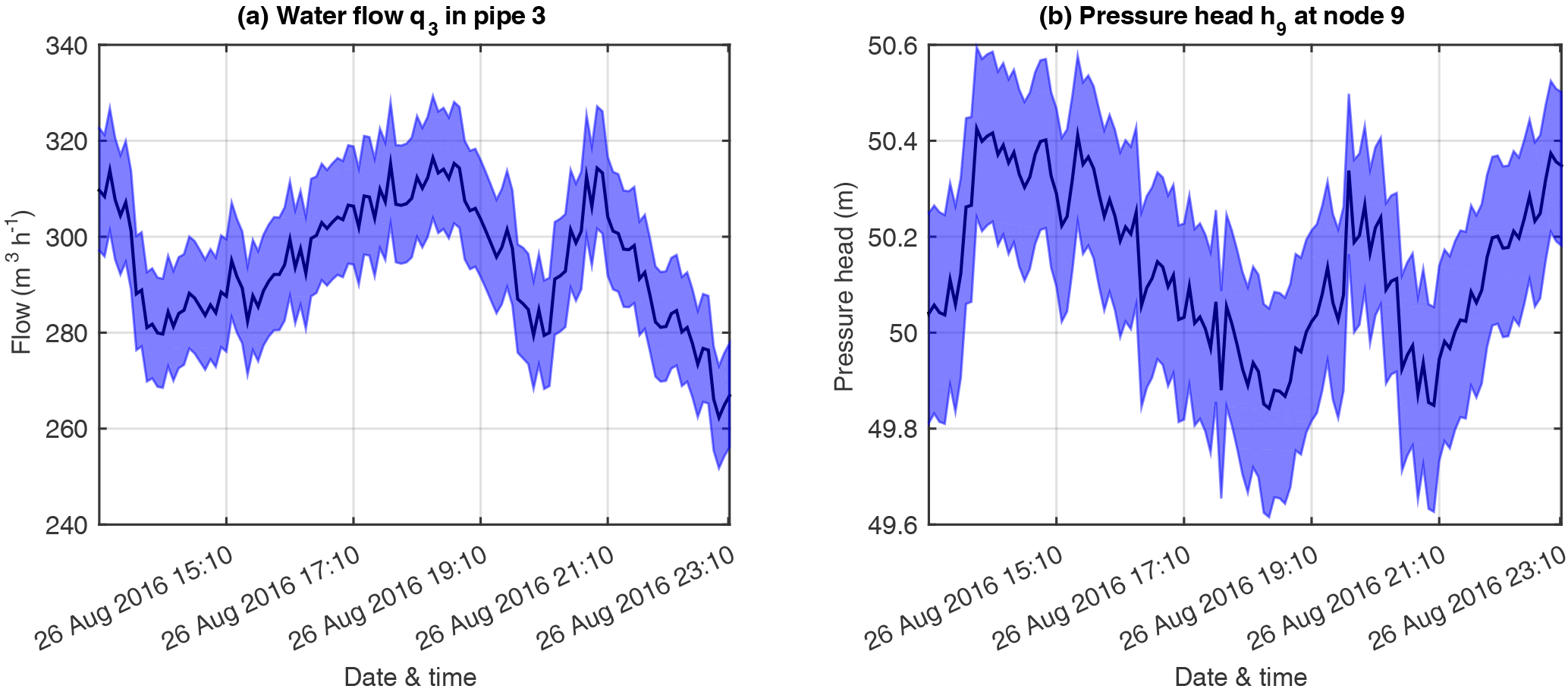
Figure 3State estimate (black line) and bounds on this estimate using the IHISE algorithm (blue area) for the water flow in pipe 3 (a) and the head at node 9 (b).
3.2 Determining the existence of unaccounted-for water using bounds on state estimates
A common practice in water utilities is to use mass balance to determine whether there is unaccounted-for water exiting the network. In this case study, since there is no sensor measuring the tank outflow q1, mass balance can be checked by generating an estimate of q1 using two different sets of data: the first is by calculating the sum of all the measured outflow (demands), indicated here by ; the second is the calculation of the tank outflow using the measured tank inflow q0(k) and tank water level measurement ht(k), indicated here by , as follows:
where αt is the base area of the tank and Δt=5 min is the measurement time step.
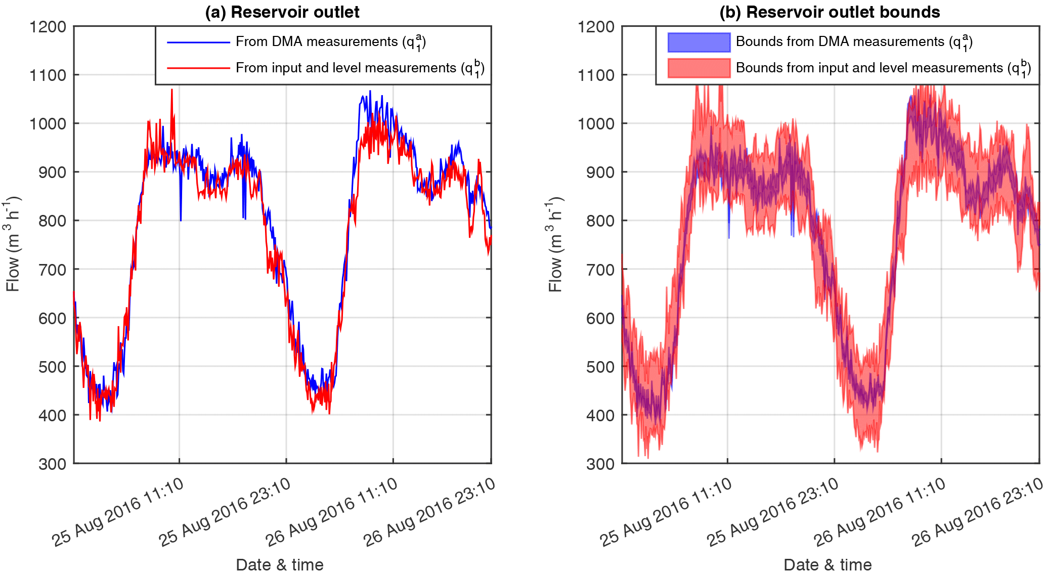
Figure 4(a) Comparison of two estimates of the tank outflow, and . (b) Comparison of the uncertainty bounds generated by the IHISE algorithm for the same estimates.
Using data from the case study network, the two tank outflow estimates were calculated for a period of 2 days, from “24 August 2016 23:10” to “26 August 2016 23:10”. The two estimates are compared in Fig. 4a. It can be observed that the two estimates have a non-zero difference at almost all time steps. This can be due to noisy data, and thus it cannot be determined with certainty whether there is unaccounted-for water. A way to deal with this is to calculate the average difference ed between these data for the given period of time, i.e., ed = mean, where ks is the total number of measurements from each sensor. This calculation gives a constant unaccounted-for flow ed=18.82 (m3 h−1), which may be due to background leakages, or it may be due to non-uniformly distributed measurement errors. Checking the water utility leakage reports of the examined period, there was no recorded leakage for the sub-network of this study.
Using the IHISE algorithm and the given model and measurement uncertainties, bounds on these same estimates can be calculated: the bounds on tank outflow by simulating the network using the network outflow and tank level measurements are indicated by , and bounds on tank outflow using the tank inflow and tank level measurements are indicated by . The comparison of these two sets of bounds is shown in Fig. 4b. The two sets of bounds overlap, indicating that the variance can be explained by measurement and modeling uncertainty. There are some specific time steps that the bounds do not overlap, which may be due to noisy data that can be eliminated using a suitable data validation strategy. It can also be observed that bounds generated by the tank level and tank inflow measurements are wider. This is because these bounds are calculated using the dynamic equation Eq. (3) which uses three uncertain measurements for the calculation of the bounds.
3.3 Determining the existence of an artificial leakage using bounds on state estimates
In this section the potential of the IHISE algorithm to be used for event detection in water distribution systems is demonstrated. An artificial leakage is added to the network model, an approximate location of which is indicated in Fig. 2. The leakage has a magnitude of 20 (m3 h−1) and its time profile is described by an abrupt constant outflow starting at “26 August 2016 00:10”.
In order to determine the location of the leak, additional measurements should be available. Assuming the existence of pressure sensors in the network, a comparison of the measured pressure with the estimated pressure could indicate the presence of a leak. However, in this case, the measurements are affected by not only the sensor uncertainty (as when calculating mass balance), but also by the network modeling uncertainty, which may greatly affect the pressure estimates. Using the IHISE algorithm, the effect of both measurement and modeling uncertainties is considered in calculating the bounding estimates, and the existence of a leak can be determined with greater certainty.
We assume the existence of a pressure sensor at node 9 of the network as shown in Fig. 2. The pressure sensor reading is compared with the IHISE bounding estimates, as shown in Fig. 5a. The error between the pressure sensor reading and the estimated bounds, which is defined as the distance of the reading from the bounds when the reading is outside the bounds, is also calculated, and is shown in Fig. 5. It is observed that there is a pressure sensor reading error after the leakage occurs. The error presents only during the night hours, when the pressure is higher due to the low demand and thus a pressure drop due to a leakage is more apparent. Similarly, if we assume the existence of a flow sensor on pipe 12, the same effect can be observed when the flow reading is compared with the IHISE bounds, as shown in Fig. 5b. There is a flow sensor error during the night hours, while the error persists in smaller magnitude for the rest of the day. These observations indicate the existence of the leakage despite the measurement and modeling uncertainties in the network.
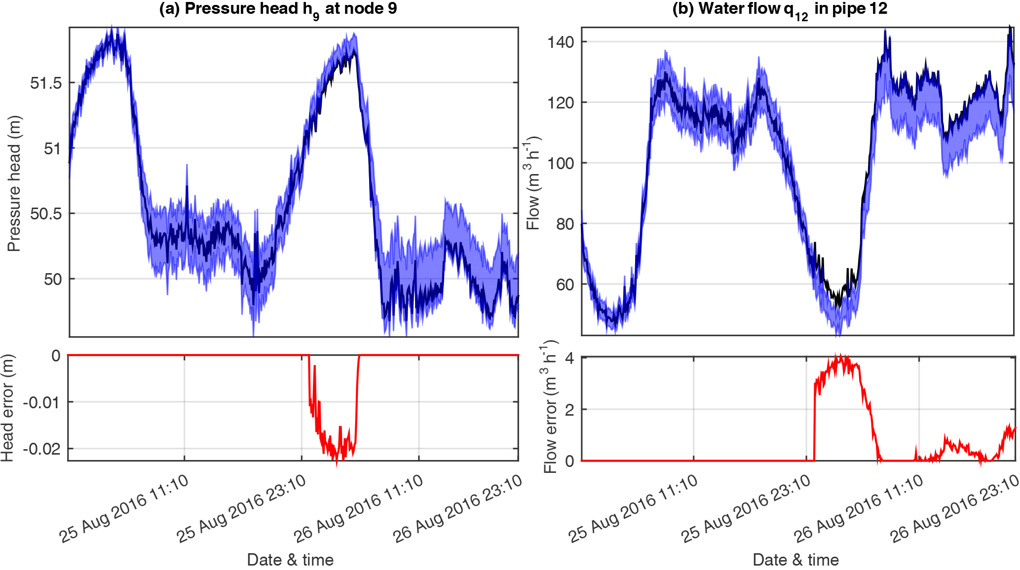
Figure 5The effect of a leakage occurring in the network at time “26 August 2016 00:10” on a pressure (a) and a flow (b) state, compared to the estimated uncertainty bounds for the same states calculated by the IHISE algorithm. Below each graph, the corresponding error of the state compared to the calculated bounds is presented.
In this work we described a methodology for real-time hydraulic interval state estimation, to monitor water transport networks. Using real-time uncertain measurements from a real transport network, the proposed Iterative Hydraulic Interval State Estimation (IHISE) algorithm generates bounds on hydraulic states of the network, by taking into account the measurement uncertainty and modeling uncertainty in the form of uncertain pipe parameters. The applicability of this methodology is demonstrated by using it to determine the existence of unaccounted-for water in the network and also to detect an artificially created leakage. Extension of this work will use the generated bounds to apply fault-diagnosis methods to localize leakages in the network. Additionally, the bounds on hydraulic states of the network will be used to generate bounds on water quality states, since the dynamics of hydraulic and quality states of a water network are interconnected.
The EPANET file for the network depicted in Fig. 2, with realistic water demands, can be found in https://doi.org/10.5281/zenodo.1185136.
The authors declare that they have no conflict of interest.
This research is funded by the European 80 Research Council under ERC
Advanced Grant ERC-2011-AdG-291508 (FAULT-ADAPTIVE) and the European Union
Horizon 2020 programme under grant agreement no. 739551 (KIOS
CoE).
Edited by: Ran Shang
Reviewed by: two anonymous referees
Andersen, J. H. and Powell, R. S.: Implicit state-estimation technique for water network monitoring, Urban Water J., 2, 123–130, 2000. a
Andersen, J. H., Powell, R. S., and Marsh, J. F.: Constrained state estimation with applications in water distribution network monitoring, Int. J. Syst. Sci., 32, 807–816, 2001. a
Bargiela, A. and Hainsworth, G. D.: Pressure and flow uncertainty in water systems, Water Resour. Plann. Manage., 115, 212–229, 1989. a
Boulos, P. F., Lansey, K. E., and Karney, B. W.: Comprehensive water distribution systems analysis handbook for engineers and planners, American Water Works Association, 2006. a
Davidson, J. W. and Bouchart, F. J.: Adjusting nodal demands in SCADA constrained real-time water distribution network models, J. Hydraul. Eng., 132, 102–110, 2006. a
Eliades, D. G., Stavrou, D., Vrachimis, S. G., Panayiotou, C. G., and Polycarpou, M. M.: Contamination event detection using multi-level thresholds, in: Proceedings of 13th Computing and Control for the Water Industry Conference, CCWI 2015, 119, 1429–1438, 2015. a
Gabrys, B. and Bargiela, A.: Integrated neural based system for state estimation and confidence limit analysis in water networks, in: Proceedings of European Simulation Symposium ESS'96, 398–402, 1997. a
Hutton, C. J., Kapelan, Z., Vamvakeridou-Lyroudia, L., and Savic, D. A.: Dealing with uncertainty in water distribution system models : A framework for real-time modeling and data assimilation, Water Resour. Plann. Manage., 140, 169–183, 2014. a
Kang, D. and Lansey, K.: Demand and roughness estimation in water distribution systems, Water Resour. Plann. Manage., 137, 20–30, 2011. a
Kang, D. S., Pasha, M. F., and Lansey, K.: Approximate methods for uncertainty analysis of water distribution systems, Urban Water J., 6, 233–249, 2009. a
Kolev, L. V.: A method for outer interval solution of parametrized systems of linear interval equations, Reliab. Comput., 10, 227–239, 2004a. a
Kolev, L. V.: An improved interval linearization for solving nonlinear problems, Numer. Algorithms, 37, 213–224, 2004b. a
Kolev, L. V.: Parameterized solution of linear interval parametric systems, Appl. Math. Comput., 246, 229–246, 2014. a, b
Savic, D. A., Kapelan, Z. S., and Jonkergouw, P. M.: Quo vadis water distribution model calibration?, Urban Water J., 6, 3–22, 2009. a
Todini, E. and Pilati, S.: A gradient algorithm for the analysis of pipe networks, in: Proceedings of International Conference on Computer Applications for Water Supply and Distribution, 1–20, 1987. a
Vrachimis, S. G., Eliades, D. G., and Polycarpou, M. M.: The backtracking uncertainty bounding algorithm for chlorine sensor fault detection, in: Proceedings of 13th Computing and Control for the Water Industry Conference, CCWI 2015, 119, 613–622, 2015. a
Vrachimis, S. G.: Dataset for “Real-Time Hydraulic Interval State Estimation for Water Transport Networks: a Case Study”, Zenodo, https://doi.org/10.5281/zenodo.1185136, 27 February, 2018.